Subcortical-cortical dynamical states of the human brain and their breakdown in stroke

 Have you doctors EXACTLY EXPLAIN to you how this is going to get you to 100% recovery. No explanation, fire your doctors, they are working for you and if they don't know how to get you 100% recovered they are not worth seeing.

Subcortical-cortical dynamical states of the human brain and their breakdown in stroke

• Chiara Favaretto,
• Michele Allegra,
• Gustavo Deco,
• Nicholas V. Metcalf,
• Joseph C. Griffis,
• Gordon L. Shulman,
• Andrea Brovelli &
• Maurizio Corbetta 

Nature Communications volume 13, Article number: 5069 (2022) Cite this article

• 8 Altmetric

• Metrics details

Abstract

The mechanisms controlling dynamical patterns in spontaneous brain activity are poorly understood. Here, we provide evidence that cortical dynamics in the ultra-slow frequency range (<0.01–0.1 Hz) requires intact cortical-subcortical communication. Using functional magnetic resonance imaging (fMRI) at rest, we identify Dynamic Functional States (DFSs), transient but recurrent clusters of cortical and subcortical regions synchronizing at ultra-slow frequencies. We observe that shifts in cortical clusters are temporally coincident with shifts in subcortical clusters, with cortical regions flexibly synchronizing with either limbic regions (hippocampus/amygdala), or subcortical nuclei (thalamus/basal ganglia). Focal lesions induced by stroke, especially those damaging white matter connections between basal ganglia/thalamus and cortex, provoke anomalies in the fraction times, dwell times, and transitions between DFSs, causing a bias toward abnormal network integration. Dynamical anomalies observed 2 weeks after stroke recover in time and contribute to explaining neurological impairment and long-term outcome.

Introduction

In the healthy brain, neuronal populations interact at multiple temporal scales, from hundreds of milliseconds to tens of seconds through interlocked rhythms^1,2,3,4. While neuroscience has traditionally focused on fast neural spiking activity^5,6, more recent theoretical work and simultaneous recordings from thousands of neurons show that activity in the infra-slow frequency range (<0.1 Hz) recruits the majority of the brain’s energy budget^7,8,9, and is behaviorally relevant^10,11,12,13. In the human brain, infra-slow fluctuations can be easily measured with fMRI blood oxygenation level-dependent (BOLD) and EEG/MEG signals¹⁴. Infra-slow activity is organized in distinct spatiotemporal patterns known as resting state networks, formed by groups of regions showing temporally correlated activity (functional connectivity, FC) and co-activating during behavioral tasks^15,16. More recently, it has been shown that this network structure reflects the long-time average (‘static FC’) of rapidly switching connectivity patterns (‘dynamic FC’ or dFC) which can be consistently observed with different analysis methods^17,18,19 and are significantly correlated with global behavioral traits (e.g. processing speed or fluid intelligence¹). The mechanisms controlling the large-scale temporal coordination of infra-slow activity are unclear, particularly whether specific regions play a leading role in orchestrating global changes in connectivity patterns. A leading hypothesis is that shifts in brain states at rest, or during tasks, depend on highly interconnected cortical regions (hubs), e.g., precuneus, posterior cingulate cortex, and lateral prefrontal cortex, that flexibly interact at different points in time with different networks^20,21,22. However, recent studies have also shown hubs in subcortical regions (basal ganglia²³, thalamus^23,24, hippocampus^20,25,26,27). Whether cortical synchronization also relies on subcortical regions is still poorly known. Clinical work has shown FC dynamics alterations in a variety of non-focal conditions (neurodegeneration, consciousness abnormalities, schizophrenia, autism)^{17,19,28,29,30,31}, which suggests that even more pronounced alterations should occur in focal conditions. Focal lesions, such as those induced by stroke, provide an ideal testbed to study the relations between brain structure and dynamics, since they considerably amplify the natural range of inter-subject variability in anatomical as well as functional connectivity. Subcortical lesions produce widespread functional alterations of the ‘static’ network structure—an anomalous inter-hemispheric segregation and intra-hemispheric integration^32,33,34. Recent studies indicate that lesions induce anomalies also at the dFC level, altering the dynamic balance between integration and segregation^35,36,37. However, which structural changes determine these functional anomalies, and how the interplay between cortex and subcortex contributes to them, has never been thoroughly investigated.

In this work, we analyze dFC patterns (“dynamic functional states” or DFSs) in a large cohort of first-time stroke patients at different clinical stages. Our study has three aims. First, we wish to describe DFSs both at the cortical and subcortical level and determine whether cortical and subcortical state dynamics are linked. Second, we examine the relation between structural lesions and alterations of FC dynamics, in terms of the fraction times and dwell times of DFSs. We use machine learning methods to explain abnormalities of dynamic FC with lesion location and patterns of structural disconnection, either at the cortical or subcortical level^34,38,39 or in cortical-subcortical pathways^27,40,41. Finally, guided by previous results on the behavioral relevance of lesion location^38,42, structural disconnections^34,42, and static FC abnormalities^33,43, we test whether information about FC dynamics enhances explanation of behavioral deficits and acute-to-chronic explanation of behavioral recovery.

Results

Definition of dynamic functional states

Control and stroke subjects were identified from the Washington University Stroke cohort (https://cnda.wustl.edu/app/template/Login). To obtain reliable dFC estimates at the individual level, we analyzed only subjects with at least 300 TR (600 s) of valid signals after pre-processing and censoring. This criterion identified 20 controls with two scan sessions 3 months apart, and 47 patients with first-time strokes with scans at three time points (2 weeks, 3 months, 12 months). The lesions frequency map of the stroke group shows that most lesions involve the deep middle cerebral artery distribution with damage of the basal ganglia and subcortical white matter (SI-Fig. 1). Fewer than 20% were cortical lesions. This distribution matches previous prospective cohorts of stroke lesions^38,44,45 (SI-Tables 1–3).

We analyzed dFC through the most straightforward approach: the sliding-window temporal correlation (window width = 60 s, window step = 2 s) followed by eigenvector decomposition and clustering (see “Methods” section and Fig. 1 for flowchart) to define a set of connectivity states that continuously activate and deactivate over time (DFSs), as in refs. 46,47,48. All projected data from controls (CTRs) and patients (PATs) (at all time points) were concatenated and clustered in time (with K-means algorithm), yielding a limited number of DFSs. We ran K-means between K = 2 and K = 10. The optimal solution was K = 5 selected through Silhouette and Davies-Bouldin indexes (SI-Fig. 2). We performed several control analyses to ensure their robustness both in terms of the size of the temporal window used for the calculation, and the number of states (K=2÷10

). We also showed that the DFSs were representative, in each window, of the dynamic FC from which they were derived (see SI paragraph S1–S4, S6 and SI-Figs. 3–7, SI-Fig. 11).

Fig. 1: Methods (dynamical functional states).

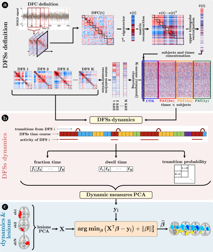
a Definition of the dynamic functional states (DFSs): (i) at first, the time course of each subject was divided into 270 time-windows of width = 30 TR (600 s) and step = 1 TR. The z-Fisher transform of the Pearson’s correlation coefficient among regions was computed at each sliding window, to estimate the Dynamical Functional Connectivity (DFC). Then, (ii) each DFC matrix was approximated by projecting on the leading eigenspace defined by the first eigenvector vi

. As the eigenvectors are defined less than the sign, we avoided this issue by reconstructing the square matrix vi×vTi. After that, (iii) the upper triangular part of these rank-one DFC matrices was vectorized and concatenated across windows and subjects, in order to finally apply a time-wise K-means clustering algorithm with correlation distance and 20 replicates (iv) to define a set of K spatial DFSs. Silhouette and Davies-Bouldin algorithms were used to search for the optimal number of DFSs. Several choices of K (from 2 to 10) were used for supplementary analyses and comparisons. b The K-means clustering associated each sliding window to a specific DFS, thus for each subject we obtained a discrete time series x(n)

, with n = 1,…, 270, where each discrete value (between 1 and K) indicated the active state at that time point. From these time courses it was possible to evaluate three different dynamical measures for each state, namely the fraction time, the dwell time, and the transition probability. To analyze the relationship among dynamical measures in healthy condition, we performed a Principal Component Analysis (PCA) over all the dynamical measures. c The projection of the sub-acute patients’ dynamical measures onto the PCs space, and the anatomical brains lesions were used as input for a Ridge Regression algorithm, aimed at identifying the lesion’s location that better characterized specific dynamic impairments. A similar approach has been used with structural disconnections.

Full size image

Dynamic functional states (DFSs) capture cortical and subcortical interactions

Five DFSs described the dynamic functional connectivity changes in healthy controls and stroke patients. We used several representations to illustrate these functional states in cortical and subcortical regions.

Figure 2 visualizes DFSs in matrix form (Fig. 2a) and through a circular graph representation (Fig. 2b). Positive weights indicate positive co-modulation, whereas negative weights indicate negative co-modulation between brain regions. We characterized DFSs in terms of the most common static FC biomarkers observed in stroke^32,34,43, namely: (1) the average homotopic inter-hemispheric connectivity (2) the average intra-hemispheric connectivity between task-positive (DAN) and task-negative (DMN) regions, as a measure of network integration (3) the overall Newman’s modularity among cortical networks, as a measure of segregation (Fig. 2c).

Fig. 2: Dynamic functional states (DFSs).

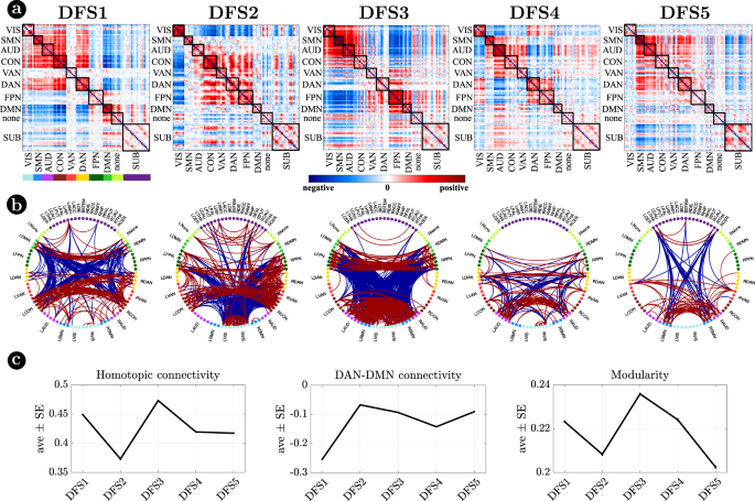
a Representation of the 5 DFSs in matrix form (positive and negative weights are red and blue, respectively). b The same DFSs are described through a circular graph representation. In each column, the positive (red) and negative (blue) strongest links for each state are represented. Network belonging is color-coded. c Average and standard error of (left) the average homotopic inter-hemispheric connectivity within each network; (center) the average connectivity between dorsal attention network (DAN) and the default mode network (DMN) regions, as a measure of task-positive and task-negative network integration); (right) the overall Newman’s modularity among cortical networks. Data are reported as mean values +/− SEM. Source data are provided as a Source data file.

Full size image

Figure 3 focuses on cortico-subcortical interactions, which are illustrated either with subcortical regions vs. cortical networks in matrix form (Fig. 3a), or as brain surface/volume maps (for cortical/subcortical regions respectively) plotting the first eigenvector of each DFS (Fig. 3b). To facilitate analysis of cortico-subcortical interactions, we performed principal component analysis (PCA) on the leading eigenvector of subcortical connectivity, identifying two main subcortical components (SCs): SC1 loads on cerebellum and subcortical nuclei: thalamus, caudate, putamen, nucleus accumbens, and globus pallidus. SC2 loads on ‘limbic’ regions like amygdala and hippocampus. By construction, these two components are not correlated. Moreover, they always correlate in opposite directions with different cortical networks.

Fig. 3: Cortico-subcortical interaction in the dynamic functional states (DFSs).

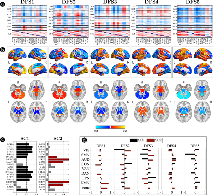
a Matrix representation of cortico-subcortical interaction. This is a zoom of Fig. 2a. Positive and negative values are indicated with red and blue, respectively. b Surface and volume projection of the first eigenvector of each DFSs. Cortical regions are shown in surface (top), while subcortical regions in volume (bottom). c Loading of each subcortical regions in the two main subcortical components. A threshold of 0.2 has been used. d Average connectivity between each subcortical component (SC1 and SC2) with each cortical network in the different DFSs. Source data are provided as a Source data file.

Full size image

Each DFS is characterized by a different set of cortical and cortical-subcortical interactions. Herein, we provide a description of each state based on these criteria. DFS1 is very similar to the healthy static FC, with high homotopic connectivity (ρz=0.45±0.0013

, where ρz indicates correlation coefficient after z-Fisher transformation), large negative DAN-DMN connectivity (ρz=−0.25±0.002), and high modularity (0.22±0.0006

). Sensory-motor-attention networks (visual: VIS, sensorimotor: SMN, auditory: AUD; control: CON, dorsal attention: DAN) are positively correlated, and negatively correlated with the default mode network (DMN) (Fig. 2a). These patterns correspond to the well-known separation between task-negative and task-positive networks⁴⁹. In-between stand high-level cognitive networks, such as the ventral attention (VAN) and fronto parietal network (FPN) that are weakly correlated with either task-positive or task-negative networks, and are expected to exhibit more flexible interactions and more individual variability^50,51. When we consider cortical-subcortical interactions, DFS1 is characterized by a positive correlation between DMN and limbic nuclei, SC2 (Fig. 3a, b), which in turn are negatively correlated with sensory-motor-attention networks.

DFS2 is very similar to the ‘pathological’ static FC observed in stroke, with low homotopic connectivity (ρz=0.37±0.002

), nearly zero DAN-DMN connectivity (ρz=−0.07±0.002), and low modularity (0.21±0.0007

). This state is characterized by a strong integration of cognitive networks (DAN, VAN, CON, FPN) and a strong negative coupling of the VIS network with other networks. AUD, SMN, and DMN maintain strong internal correlation, but remain relatively independent.

DFS3 is characterized by a high homotopic connectivity (ρz=0.47±0.0014

) and a high modularity (0.24±0.0006), similar to DFS1. However, it does not show a strong (negative) correlation between DAN and DMN (ρz=−0.09±0.002

). Instead, it captures a negative correlation between a sensory-motor cluster (VIS, SMN, AUD) and a cognitive cluster (FPN, DMN, DAN, VAN). Like DFS1, DFS3 is characterized cortically by the well-known segregation between sensory-motor networks (VIS-AUD-SMN) and DMN. However, cortico-subcortical interactions are very different in the two states: the coupling pattern between SC1–SC2 and sensorimotor/DMN is opposite. SC2 (limbic) correlates positively with the DMN in DFS1, but negatively in DFS3. Correspondingly, SC2 shows no correlation with sensory-motor networks in DFS1, but a positive correlation in DFS3. In contrast, SC1 (nuclei) shows no correlation with DMN in DFS1, but a positive correlation with DMN and a negative correlation with sensory-motor networks in DFS3 (Fig. 3c, d).

DFS4 shows intermediate values of homotopic connectivity (ρz=0.42±0.0014

), DAN-DMN connectivity (ρz=−0.14±0.002), and modularity (0.22±0.0006

). In this state, we observe anti-correlation between a VIS-DAN-FPN cluster and a SMN-AUD-CON-VAN-DMN cluster. Interestingly, in DFS4 all subcortical regions show positive correlation and appear strongly uncorrelated from cortex.

Finally, DFS5 shows intermediate values of homotopic (ρz=0.42±0.0015

) and DAN-DMN (ρz=−0.09±0.002) connectivity, and a very low value of modularity (0.20±0.0007

). Indeed, it reflects another state of integration among almost all networks (like DFS2), except VIS and DMN that remain more segregated. DFS5 differs from DFS2 for the absence of the negative correlation between VIS and all other networks.

In summary, we identified a set of spatial maps of inter-regional correlation alternating over time (DFSs) characterized by different cortical and subcortical connectivity patterns. An important insight is that, in each DFS, different cortical clusters connect with a specific set of subcortical nuclei (Fig. 3a, b). In fact, changes in cortical states were temporally coincident with shifts in subcortical connectivity. Figure 4a shows exemplar time courses of the leading eigenvector of cortical connectivity, projected onto different networks (top), and the two principal components of the leading eigenvector of subcortical connectivity (bottom), during switch between DFSs. Coincident cortico-subcortical reorganization is plainly appreciable. Importantly, the reorganization of subcortical and cortical patterns was generally synchronized irrespective of the definition of a DFS switch. Indeed, we evaluated connectivity shifts, defined as connectivity differences between pairs of consecutive sliding windows, separately for cortical and subcortical regions. We found that subcortical shifts were positively correlated with network cortical shifts (all correlations >0.5

). Both cortical and subcortical connectivity shifts showed (in absolute value) a heavy tail distribution, with more frequent low differences (Fig. 4b left). Thus, we defined a jump when a large connectivity difference occurred (0.29, corresponding to the top 5% values). Then, we tested the simultaneity of cortical and subcortical reorganization by comparing the probability that cortical and subcortical jumps occur simultaneously (estimated as P(subcorticalchanges|corticalchanges)) under the null hypothesis of independent processes, and in the observed data (see “Methods” for details on this analysis). We evaluated these measures for each subject, and we compared the two distributions through the Wilcoxon rank test. For all networks, we found that the observed conditioned probability was significantly larger than the probability under the null hypothesis (all p<10−40

, Bonferroni corrected for 9 networks), supporting the idea of synchronous cortical and subcortical shifts (Fig. 4b right). It is important to highlight that in this analysis we considered all sliding windows, not just those defining DFS boundaries. Therefore, the time course synchronization analysis was independent of the DFS definition.

Fig. 4: Cortical and subcortical dynamics.

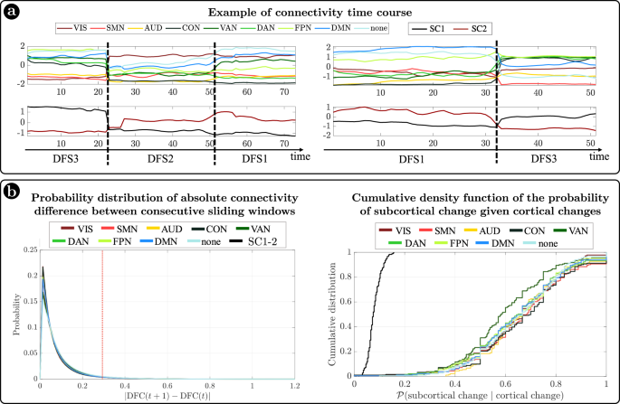
a Two examples of average connectivity during time for cortical networks (top) and subcortical clusters (bottom). The vertical dashed lines indicate the switching between dynamic functional states (DFSs). b (Left) Probability distribution of the absolute values of connectivity differences between consecutive sliding windows. Each line represents a different network. Right) Cumulative density function of the conditioned probability of subcortical connectivity reorganization, given a cortical connectivity reorganization. Each colored line relates to a different cortical network. The black line shows the cumulative density function under the null hypothesis of independence between cortical and subcortical changes. Source data are provided as a Source data file.

Full size image

Importantly, the observed coordination between cortical and subcortical dynamics does not depend on the specific subcortical parcellation used. We replicated our original analyses (based on the Freesurfer parcellation) with a more recent subcortical parcellation⁵². Tian et al.⁵² developed four subcortical parcellations with increasing levels of resolution (16, 32, 50, or 54 regions, respectively). We limited our analysis to the lowest (16 regions) and highest (54 regions) resolution parcellations. Detailed results are presented in the Supplementary Information (SI paragraph S7 and SI-Figs. 12, 13). The choice of parcellation did not influence our three main findings: (1) the ‘antagonistic’ dynamics of basal ganglia vs limbic regions, represented by two anticorrelated principal components of subcortical dynamic FC; (2) the observation that different DFS are associated with different patterns of cortical/subcortical interactions, as shown by different patterns of connectivity between the main subcortical clusters and cortical networks; and (3) the coordination between cortical and subcortical dynamics, as shown by simultaneous cortical/subcortical FC shifts. Qualitatively, the main difference between results in the two parcellations is related to the thalamus. While in the Freesurfer parcellation, used in the original analysis, the thalamus essentially grouped with the basal ganglia, the new parcellation yields a more nuanced picture, hinting at a functional split between different parts of the thalamus: the anterior portion of the thalamus groups with the basal ganglia, whereas the posterior portion cannot be clearly affiliated to either of the two clusters (basal ganglia/limbic). A fine-grained analysis of the relation between thalamic nuclei and DFS is left for future work.

Sub-acute stroke causes a DFS imbalance with a bias toward integration that recovers over time

DFSs imbalance in stroke patients

Next, we employed dynamical measures related to the alternation of DFSs to study how stroke lesions affect these dynamic features (“Methods”, Fig. 1). By construction, only one DFS can be active in each sliding window. Therefore, the dynamic of the functional connections can be described in terms of a single time series of discrete values (from 1 to 5), each associated to a DFS. Three measures were extracted to characterize the dynamic of DFSs, namely the fraction time (f

), the dwell time (ℓ

) and the transition probability (e.g., transition from DFS1 to DFS2: DFS1>2), which describe the number of times each state is active, the duration of each state and the probability to switch from one state to another (“Methods” and Fig. 1 for details), respectively.

The characterization of DFSs in terms of the most common static FC stroke biomarkers suggest that DFSs alterations may be more sensitively detected in patients with more severe static FC impairment. Accordingly, we divided stroke patients with severe or mild static (average) FC impairment at 2 weeks and performed all dynamic analyses with three groups: healthy controls, stroke patients with severe or mild FC impairment at 2 weeks. To that effect, we performed a spatial PCA to find a component summarizing the static FC abnormalities explaining the largest portion of variance over patients. To avoid biases in patient selection, this PCA was run in an independent sample of 67 sub-acute patients not suitable for the dynamic analysis. The weights of this summary component (ST) identified two groups of patients: with more severe (ST > 0) (n = 18) or milder (ST < 0) (n = 29)) static FC changes (for details SI paragraph S8 and SI-Fig. 15). In what follows, we will refer to these two groups as ‘severe’ and ‘mild’ patients, as patients with ST > 0 were overall more severe in their neurological impairment than patients with ST < 0 (mean NIHSS score: 7.23 (ST > 0) vs 2.37 (ST < 0); t test: T = 4.02, p = 2.6 × 10⁻⁴) as shown in SI paragraph S8. The main dynamical difference between control subjects and sub-acute patients was the fraction time (f

) of the different DFSs (Fig. 5a top graphs). The control population showed a uniform distribution of DFSs’ fraction time, with the exception of DFS5, which was significantly less frequent than all the other states except DFS4, as assessed through a non-parametric permutation test (mean ± standard error: f1=0.25±0.03; f2=0.22±0.03; f3=0.23±0.02; f4=0.18±0.02; f5=0.11±0.01; f5<f1 (t=−4.25), f5<f2 (t=−3.50), f5<f3 (t=−4.50): all p=10−3, Bonferroni corrected). Similarly, the dwell time (ℓ) was similar across all DFS except for a significantly longer duration of DFS1 as compared to DFS5 (ℓ1>ℓ5, t=3.23,p=0.02, Bonferroni corrected) (mean ± standard error: ℓ1=13.97±1.44TR; ℓ2=12.16±1.46TR; ℓ3=12.59±1.13TR; ℓ4=12.47±1.24TR; ℓ5=8.40±0.89TR

).

Fig. 5: Results.

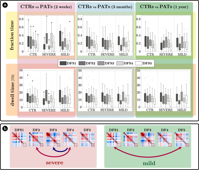
a Fraction time and lifespan. This figure represents two dynamical measures related to the dynamic functional states (DFSs), namely the fraction time (top) and the average dwell time (bottom). Comparisons between healthy controls (CTRs) and stroke patients (PATs) at different conditions are represented. To be noticed: (i) fraction times and dwell times show similar patterns, but fraction times are more sensitive to identify group differences, and (ii) all dynamic impairments identified at the sub-acute stage, recovered in the chronic stage. The significance between each pair of groups has been tested independently for each of the 5 DFSs through one-sided non-parametric permutation tests, and false discovery rate (FDR) correction for 15 comparisons. The symbol * indicates p-value < 0.05 after FDR correction. For each panel: n = 40 (CTRs), 18 (PATs severe), 29 (PATs mild). On each box: the central green line indicates the median, the red cross indicates the mean, and the bottom and top edges of the box indicate the 25th and 75th percentiles, respectively. The whiskers extend to the most extreme data points, not considered outliers (plotted individually using a dot). b Graphical representation of the significant differences in transition probabilities between CTRs and patients at the sub-acute stage: red arrows represent increase in probability, while blue arrows stand for decreased transition probabilities. Source data are provided as a Source data file.

Full size image

We tested the effect of DFSs and groups (controls, sub-acute severe patients, and sub-acute mild patients) in the fraction times through a generalized linear mixed effect model (GLME) with Poisson distribution, with DFS and group as factors. We found a significant interaction effect (F=211.13,p=0

) and both single main effects of DFSs (F=151.95,p=0) and groups (F=168.29,p=0). Note that this result may be affected by collinearity, as fraction times for different DFS are not independent. However, we conducted post hoc analyses for each DFS separately (with non-parametric permutation tests), finding two different patterns of abnormalities for severe and mild patients. Severe patients manifested an abnormal increase of DFS2 (f2=0.36±0.06; t=2.30,p=0.02, FDR corrected for 15 comparisons) and marginally DFS4 (f4=0.28±0.05; t=1.84,p=0.051, FDR corrected), at the expense of DFS1 (f1=0.13±0.02) and DFS3 (f3=0.11±0.02) that were significantly less frequent than in CTRs (DFS1: t=−3.50,p=0.003 FDR corrected; DFS3: t=−4.53,p=0.0003, FDR corrected). Therefore, severe patients had an anomalous under-expression of segregated states 1 and 3 and overexpression of integrated state 2. In contrast, mild patients showed an imbalance between the two integrated states, with an abnormal increase of DFS5 (f5=0.20±0.04; t=2.20,p=0.024, FDR corrected for 15 comparisons) occurrences, and an anomalous decrease in DFS2 (f2=0.15±0.02; t=1.98,p=0.046

, FDR corrected). In general, measures of dwell time (Fig. 5a bottom graphs) replicated the patterns observed with fraction time but were less sensitive.

Fraction time and dwell time measures do not consider dynamical switches among DFSs that are defined by the transition probability (Fig. 5b). We found a significant interaction (F=2.99,p<10−8

) and a main effect of transitions (F=1.83,p=0.015) through a GLME with Normal distribution. As compared to controls, more severe sub-acute patients were characterized by more frequent bidirectional transitions between DFS4 and DFS2 (DFS2>4: t=3.16,p=0.004; DFS4>2: t=3.20,p=0.004, FDR corrected for 20 comparisons), and fewer transitions from DFS4 to DFS3 (DFS4>3: t=−3.27,p=0.004, FDR corrected). Moreover, bidirectional anomalies in transitions were found between DFS1 and DFS5 for mild patients (increased DFS1>5: t=2.25,p=0.05 and DFS5>1: t=2.50,p=0.03

, FDR corrected). In summary, the transition analysis showed that more/less frequent states in stroke are also visited more/less frequently, e.g., DFS2 for severe patients and DFS5 for mild patients. Notably, all dynamic abnormalities in fraction time, dwell time, and transition probability observed at the sub-acute stage recovered over time at 3 and 12 months (Fig. 5). In summary, more severe stroke patients are characterized by more frequent network integration states (DFS2,4), and more transitions towards them, with a corresponding decrease of network segregation states (DFS1,3). In addition, there is a clear difference between stroke patients with severe or mild FC anomalies, with the latter group preferring to spend more time in DFS5 than DFS2. Importantly, sub-acute alterations in state dynamics recovered at 3- and 12-months post-stroke.

In a control analysis (SI paragraph S5, SI-Fig. 8), we verified that these results are not a consequence of motion scrubbing. We considered both a more stringent and a more liberal scrubbing threshold (corresponding respectively to a higher and a lower number of censored frames) and we observed no qualitative impact on the results.

More at link.