Data Driven Models of Short-Term Synaptic Plasticity

No fucking clue how you could use this to create neuroplasticity on demand.  Ask your doctor how to read the equations and use this in a stroke protocol.
https://www.frontiersin.org/articles/10.3389/fncom.2018.00032/full?

Original Research ARTICLE

Front. Comput. Neurosci., 22 May 2018 | https://doi.org/10.3389/fncom.2018.00032

Elham Bayat Mokhtari¹, J. Josh Lawrence² and Emily F. Stone^1*

• ¹Department of Mathematical Sciences, The University of Montana, Missoula, MT, United States
• ²Pharmacology and Neuroscience, Texas Tech University Health Sciences Center, Lubbock, TX, United States

Simple models of short term synaptic plasticity that incorporate facilitation and/or depression have been created in abundance for different synapse types and circumstances. The analysis of these models has included computing mutual information between a stochastic input spike train and some sort of representation of the postsynaptic response. While this approach has proven useful in many contexts, for the purpose of determining the type of process underlying a stochastic output train, it ignores the ordering of the responses, leaving an important characterizing feature on the table. In this paper we use a broader class of information measures on output only, and specifically construct hidden Markov models (HMMs) (known as epsilon machines or causal state models) to differentiate between synapse type, and classify the complexity of the process. We find that the machines allow us to differentiate between processes in a way not possible by considering distributions alone. We are also able to understand these differences in terms of the dynamics of the model used to create the output response, bringing the analysis full circle. Hence this technique provides a complimentary description of the synaptic filtering process, and potentially expands the interpretation of future experimental results.

1. Introduction

Short term plasticity at the synapse level can have profound effects on functional connectivity of neurons. Through repetitive activation, the strength, or efficacy, of synaptic release of neurotransmitter can be decreased, through depletion, or increased, through facilitation. A single synapse type can display different properties at different frequencies of stimulation.

The role of synaptic plasticity and computation has been analyzed and reported on in numerous papers over the past 30 years. A review of feed-forward synaptic mechanisms and their implications can be found in Abbott and Regehr (2004). In this paper Abbott and Regher state “The potential computational power of synapses is large because their basic signal transmission properties can be affected by the history of presynaptic and postsynaptic firing in so many different ways.” They also outline the basic function of a synapse as a signal filter as follows: Synapses with an initial low probability of release act as high pass filters through facilitation, while synapses with an initially high probability of release exhibit depression and subsequently serve as low pass filters. Intermediate cases in which the synapse can act as a band-pass filter, exist. Identifying synapse-specific molecular mechanisms is currently an active area of research, involving subtle changes in expression of myriad calcium sensor isoforms (synaptotagmins), subtly configured to alter the microscopic rates of synaptic release, facilitation, depression, and vesicle replenishment (Fioravante and Regehr, 2011; Chen and Jonas, 2017; Jackman and Regehr, 2017).

The underlying mechanisms creating these effects may be inferred by fitting an a priori model to synaptic response data. We parameterize such a model combining the properties of facilitation and depression (FD) at the presynaptic neuron with experimental data from dual whole-cell recordings from a presynaptic parvalbumin-positive (PV) basket cell (BC) connected to a postsynaptic CA1 (Cornu Ammonis 1 subregion) pyramidal cell, for fixed frequency spike trains into the presynaptic PV BC (Stone et al., 2014; Lawrence et al., 2015). We later examine the response of the model to an in vivo-like Poisson spike train of input, where the inter-spike interval (ISI) follows an exponential distribution, in Bayat et al. (submitted). Here we investigate the information processing properties of the synapse in question, following (Markram et al., 1998) and using standard calculations of entropy and mutual information between the input spike train and output response. This, however, left us unsatisfied, as it did not indicate the history dependence of the response, which we believe is one of the more interesting features of plasticity models that involve presynaptic calcium concentration. We attempted using multivariate mutual information measures, but this very quickly collapses due to the “curse of dimensionality” (Bellman, 1957). In this paper we try to resolve the question using methods of Computational Mechanics, creating unifilar HMMs called epsilon machines, that represent the stochastic process that our synapse model creates. As a bonus we are using data itself (albeit synthetic data) to create models of plasticity that can be used to classify properties of different types of synapses.

As stated in the abstract, methods from Information theory rely on distribution measures which inherently ignore the ordering of the measured data stream. We seek to incorporate this important feature of plasticity, the dependence of the response of the synapse on the prior sequence of stimulation, directly through the construction of causal state machines. This can only add to the understanding of the process in cases where the input stimulus train is known. In experiments where only the output postsynaptic response is known, this technique is particularly useful. While the machines themselves cannot be interpreted in a physiological way, the information they provide can be used to classify synaptic dynamics and inform the construction of physiological models. The point of the analysis is to gain as much accurate information from experiments in short term synaptic plasticity as possible without imposing the bias of an assumed underlying physical model. To create synthetic data we use a very simple but otherwise complete model of short-term plasticity that incorporates a “memory” effect through the inclusion of calcium build-up and decay. This has roots in a real physiological process (the flooding of calcium into the presynaptic terminal can trigger the release of neurotransmitter), but we are not interested per se in creating a biophysically complete model here. The calcium dynamics simply introduces another time scale into the model, one that is physiologically relevant. We wish to explore the effect of this additional time scale on the complexity of the process.

Computational Mechanics is an area of study pioneered by Crutchfield and colleagues in the 1990s, (Crutchfield and Young, 1989; Crutchfield, 1994; Shalizi and Shalizi, 2002). Finding structure in time series with these techniques has been applied in such diverse arenas as layered solids (Varn et al., 2002), Geomagnetism (Clarke et al., 2003), climate modeling (Palmer et al., 2002), financial time series (Park et al., 2007), and more recently ecological models (Boschetti, 2008) and large scale multi-agent simulations (Parikh et al., 2016). In neuroscience, to name a few only, we note one application to spike train data (Haslinger et al., 2013), and a recent publication by Marzen et al. on the time resolution dependence of information measures of spike train data (Marzen et al., 2015).

We employ some of the simplest ideas from this body of work, namely decomposing a discrete time-discrete state data stream into causal states, which are made up of sequences of varying length that all give the same probability of predicting the same next data point in the stream. The data are discrete time by construction, and made into discrete symbols through a partition, so the process can be described by symbolic dynamics. We use the Causal State Splitting Reconstruction (CSSR) algorithm on the data to create the causal states and assemble a HMM that represents the transitions between the states, while emitting a certain symbol. This allows us to classify the synapse types and gives an idea of the differences in the history dependence of the processes as well.

Using an a priori model for short-term synaptic dynamics and fitting it to data, while a perfectly valid approach, allows only for the discovery of the parameters in the model and possibly a necessary model reduction to remove any parameter dependencies (too many parameters in the model for the data set to fit). The alternative approach is to allow the data itself to create the model. From these “data driven” models, conclusions can be drawn about the properties of the synapse that are explicitly discoverable from the experimental data. The ultimate goal is a categorization of the types of processes a synapse can create, and an assignment of those to different synapse types under varying conditions. Note that the complexity or level of biophysical detail of our model synapse is not important to this end. In fact, the best way to calibrate this method is using the simplest possible model of the dynamics that captures the history dependence of the plasticity. This is not consonant with the goal of incorporating as many physiological features as possible, whether they affect the dynamics significantly or not. In fact, in most cases the limited data in any electro-physiological experiment precludes identifying more than a handful of parameters in an a priori model, a point we discuss in Stone et al. (2014). Our goal is to classify the sort of filter the synapse creates under certain physiological conditions, rather than to identify specific detailed cellular level mechanisms.

We are motivated in this task by the work of Kohus et al. (2016), in which they present a comprehensive data set describing connectivity and synaptic dynamics of different interneuron (IN) subtypes in CA3 using paired cell recordings. They apply dynamic stimulation protocols to characterize the short-term synaptic plasticity of each synaptic connection across a wide range of presynaptic action potential frequencies. They discovered that while PV+ (parvalbumin positive) cells are depressing, CCK+ (Cholecystokinin positive) INs display a range of synaptic responses (facilitation, depression, mixed) depending upon postsynaptic target and firing rate. Classifying such a wide range of activity succinctly is clearly useful in this context. The discovery that the rate of particular observed oscillations in these cells (called sharp wave ripples) may be paced by the short-term synaptic dynamics of the PV+BC in CA3 demonstrates the importance of these dynamics in explaining complex network phenomena.

The paper is organized as follows. The construct for an experimental paper with section 2 and section 3 is not an immediately obvious partition of our work, but we use it as best we can. In the section 2 we describe the background on the synaptic plasticity model, and some analysis of its properties. We also cover the necessary background from Computational Mechanics. Finally we show how the techniques are explicitly applied to our data. In the section 3 we present the epsilon machines created from data from three types of synapses from our FD model: depressing, facilitating, and mixed, at varying input frequencies. Here we also indicate similarities and differences in the actual machines. In the section 4 we speculate on the reasons for these features by referring back to the original model. In the last section we indicate directions for future work.

2. Materials and Methods

2.1. Model of Synaptic Plasticity

In Stone et al. (2014), we parameterize a simple model of presynaptic plasticity from work by Lee et al. (2008) with experimental data from cholinergic neuromodulation of GABAergic transmission in the hippocampus. The model is based upon calcium dependent enhancement of probability of release and recovery of signalling resources (For a review of these mechanisms see Khanin et al., 2006). It is one of a long sequence of models developed from 1998 to the present, with notable contributions by Markram et al. (1998) and Dittman et al. (2000). The latter is a good exposition of the model as it pertains to various types of short term plasticity seen in the central nervous system, and the underlying dependence of the plasticity is based on physiologically relevant dynamics of calcium influx and decay within the presynaptic terminal. In our work, we use the Lee model to create a two dimensional discrete dynamical system in variables for calcium concentration in the presynaptic area and the fraction of sites that are ready to release neurotransmitter into the synaptic cleft.

In the rest of this section we outline the model, which is used to generate synthetic data for our study of causal state models, or epsilon machines, of short-term plasticity.

In the model the probability of release (P_rel) is the fraction of a pool of synapses that will release a vesicle upon the arrival of an action potential at the terminal. Following the work of Lee et al. (2008), we postulate that P_rel increases monotonically as function of calcium concentration in a sigmoidal fashion to asymptote at some P_max. The kinetics of the synaptotagmin-1 receptors that binds the incoming calcium suggests a Hill equation with coefficient 4 for this function. The half-height concentration value, K, and P_max are parameters determined from the data.

After releasing vesicles upon stimulation, some portion of the pool of synapses will not be able to release vesicles again if stimulated within some time interval, i.e., they are in a refractory state. This causes “depression;” a monotonic decay of the amplitude of the response upon repeated stimulation. The rate of recovery from the refractory state is thought to depend on the calcium concentration in the presynaptic terminal (Dittman and Regehr, 1998; Wang and Kaczmarek, 1998). The model has a simple monotonic dependence of rate of recovery on calcium concentration, a Hill equation with coefficient of 1, starting at some k_min, increasing to k_max asymptotically as the concentration increases, with a half height of K_r.

The presynaptic calcium concentration itself, [Ca], is assumed to follow first order decay kinetics to a base concentration, [Ca]_base. At this point we choose that [Ca]_base = 0, since locally (near the synaptotagmin-1 receptors) the concentration of calcium will be quite low in the absence of an action potential. The evolution equation for [Ca] then is simply τcad[Ca]dt=−[Ca]${\tau }_{ca}\frac{d\left[Ca\right]}{dt}=-\left[Ca\right]$ where τ_ca is the calcium decay time constant, measured in milliseconds. Upon pulse stimulation, presynaptic voltage-gated calcium channels open, and the concentration of calcium at the terminal increases rapidly by an amount δ (measured in μm): [Ca] → [Ca]+δ at the time of the pulse. Note that calcium build-up is possible over a train of pulses if the decay time is long enough relative to the ISI.

As mentioned above, the probability of release P_rel and the rate of recovery, k_recov, depend monotonically on the instantaneous calcium concentration via Hill equations with coefficients of 1 and 4 respectively. Rescaling the calcium concentration by δ = δ_c in the control case, we define C = [Ca]/δ_c. Then the equations are Prel=PmaxC4C4+K4,$P_{rel}=P_{max}\frac{C^4}{C^4+K^4},$ and krecov=kmin+ΔkCC+Kr$k_{recov}=k_{min}+\Delta k\frac{C}{C+K_r}$ . The variable R_rel is governed by the ordinary differential equation dRreldt=krecov(1−Rrel),$\frac{d{R}_{rel}}{dt}=k_{recov}(1-R_{rel}),$ which can be solved exactly for R_rel(t). Rrel(t)=1−(1−R0)(C0e−t+KrKr+C0)Δke−kmint$R_{rel}(t)=1-(1-R_0){(\frac{C_0{e}^{-t}+K_r}{K_r+C_0})}^{\Delta k}{e}^{-k_{min}t}$ . P_rel is also a function of time as it follows the concentration of calcium after a stimulus.

We used experiments in hippocampus to parameterize this model, as part of an exploration of the frequency dependent effects of neuromodulation. Whole-cell recordings were performed from synaptically connected pairs of neurons in mouse hippocampal slices from PV-GFP mice (Lawrence et al., 2015). The presynaptic neuron was a PV basket cell (BC) and the postsynaptic neuron was a CA1 pyramidal cell. Using short, 1–2 ms duration suprathreshold current steps to evoke action potentials in the PV BC from a resting potential of −60 mV and trains of 25 of action potentials are evoked at 5, 50, and 100 Hz from the presynaptic basket cell. The result in the postsynaptic neuron is the activation of GABA_A-mediated inhibitory postsynaptic currents (IPSCs). Upon repetitive stimulation, the amplitude of the synaptically evoked IPSC declines to a steady-state level. These experiments were conducted with 5, 50, and 100 Hz stimulation pulse trains, with and without the neuromodulator muscarine, in order to test frequency dependent short term plasticity effects.

The peak of the measured postsynaptic IPSC is presumed to be proportional to the total number of synapses that receive stimulation N_tot, which are also ready to release (R_rel), e.g., N_totR_rel, multiplied by the probability of release P_rel. That is, peak IPSC ~N_totR_relP_rel. P_rel and R_rel are both fractions of the total, and thus range between 0 and 1. Without loss of generality, we consider peak IPSC to be proportional to R_relP_rel.

From the continuous time functions describing C, R_rel, and P_rel, we constructed a discrete dynamical system (or “map”) that describes P_relR_rel upon repetitive stimulation. Given an ISI of T, the calcium concentration after a stimulus is C(T) + Δ (Δ = δ/δ_c), and the peak IPSC is proportional to P_rel(T)R_rel(T), which depend upon C. After the release, R_rel is reduced by the fraction of synapses that fired, e.g., R_rel → R_rel−P_relR_rel = R_rel(1 − P_rel). This value is used as the initial condition in the solution to the ODE for R_rel(t). A two dimensional map (in C and R_rel) from one peak value to the next is thus constructed. To simplify the formulas we let P = P_rel and R = R_rel. The map is

Cn+1=Cne−T+Δ,    (1)$\begin{array}{rc}{C}_{n+1}=C_n{e}^{-T}+\Delta ,& (1)\end{array}$

Pn+1=PmaxC4n+1C4n+1+K4,    (2)$\begin{array}{rc}{P}_{n+1}=P_{max}\frac{C_{n+1}^4}{C_{n+1}^4+K^4},& (2)\end{array}$

Rn+1=1−(1−(1−Pn)Rn)(Cne−T+KrKr+Cn)Δke−kminT.    (3)$\begin{array}{rc}{R}_{n+1}=1-(1-(1-P_n)R_n){(\frac{C_n{e}^{-T}+K_r}{K_r+C_n})}^{\Delta k}{e}^{-k_{min}T}.& (3)\end{array}$

Following this notation the peak value upon the nth stimulus is Pr_n = R_nP_n, where R_n is the value of the reserve pool before the release reduces it by the fraction (1 − P_n).

Data from the experiments were fitted to the map using the Matlab package lsqnonlin, and with Bayesian techniques (Haario et al., 2006). The value of P_max was determined by variance-mean analysis, and is 0.85 for the control data and 0.27 for the muscarine data. The common fitted parameter values for both data sets are shown in Table 1.

TABLE 1

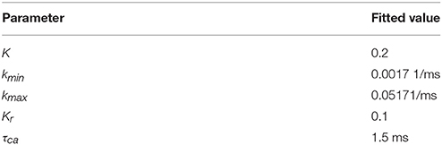Table 1. Parameter values.

For the control data set Δ = 1, and the muscarine data set has the fitted value of Δ = 0.17. From this result it is clear that the size of the spike in calcium during a stimulation event must be much reduced to fit the data from the muscarine experiments. This is in accordance with the idea that mAChR activation reduces calcium ion influx at the terminal.

Much more between here and the results. 

3. Results

Results for the depressing synapse are shown in Figure 4 and details for all these machines can be found in Appendix 1. We indicate on the histograms where the maximum statistical complexity is with a red line. For low frequencies, the probability of getting a large Pr value (or a “1”) is quite large, and its epsilon machine captures that dynamic with one state. Similarly for high frequencies the probability of getting a small Pr value (or a “0”) is quite large and a one state machine results with the probabilities reversed. For intermediate frequencies, near the maximum entropy value of 2–3 Hz, the epsilon machine has 2 states, indicating a more complicated sequence of low and high Pr-values. Both 2 and 5 Hz have identical machines in structure with slight variations in the transition probabilities.

The words in each causal state indicate the kind of sequences that are typical of the synapse. For 2 and 5 Hz, state 0 contains the sequences 00, 10, 000, 010, 100, and 110. State 1 contains 01, 11, 001, 011, 101, and 111. Between the two, all possible sequences of length 2 and 3 are represented. The probability of getting a 0 or a 1 is more or less equally likely from both states. State 0 contains more zeros overall, so it is the lower Pr state. Note that the transition from state 0 to state 1 occurs with the emission of a 1, so the occurrence of a 1 in the sequence drives the dynamic to state 1, and visa versa. This is a kind of sorting of sequences into words with more zeros and those with more 1's. There is nothing particularly “hidden” in this HMM. For us it means the dynamics of the synapse are best understood in terms of the histograms. There is nothing particularly complex in the filter produced by the map.

We have already seen that the histograms for the depressing synapse are well represented by the stochastic fixed point distribution. And even though the distribution sloshes around as the frequency is varied, there is little change in complexity in the epsilon machines through this range. There are several ways to interpret this result. One is that the very short τ_ca means there is little correlation in calcium time series, which in turn determines the correlation in P and, indirectly and directly, R. We examine this idea further in section 4. Another way is to consider the histograms themselves which are either fairly flat, or with a single peak at smaller Pr-values and an exponential type tail to the right. The structure is simple, and can be understood as a “stochastic fixed point” filter of the incoming Poisson spike train. All this is in contrast with the results for the facilitating synapse, which we show in Figure 5.

FIGURE 5

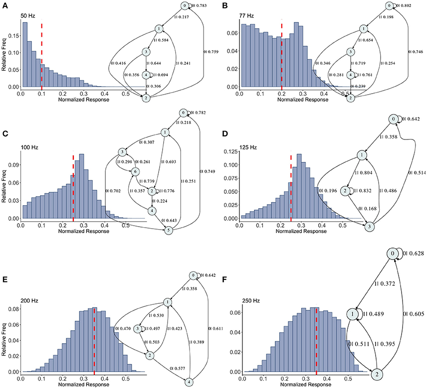
Figure 5. Causal state machines (CSMs) reconstructed and their corresponding relative frequency distributions obtained from facilitating FD model driven by Poisson spike train with mean firing rates (A) 50, (B) 77, (C)100, (D) 125, (E) 200, and (F) 250 Hz. State “0” is the baseline state. Similar graph structure is seen for mean firing rates of 50 and 70 Hz. Under mean firing rate of 100 Hz, the graph structure is more complex with more edges, vertices, and one set of parallel edges from state “3” to “6”. This increase in complexity is somewhat not surprising as this is inflection point where the concavity of the normalized response fixed point for this synapse model changes at this firing rate, (see Figure 1). In non-physiological range from 125 to 250 Hz, the complexity of graph structure decreases.

Histograms of the output Pr are shown in Figures 5A–F, for 50, 77, 100, 125, 200, 250 Hz, respectively, along with their corresponding epsilon machines of L = 3. For frequencies less than 50 Hz the machine has one state. Starting at ν = 50, all the machines can be described by referring to a persistent “inner cycle” and “outer cycle.” With the exception of the 100 Hz machine, which has a third cycle, they can be related to one another by graph operations as the frequency is varied. For instance, at 50 and 77 Hz, the machines are topologically similar, with small variations in the transition probabilities. Note however that the histograms are not similar in any obvious way; the epsilon machine identifies the underlying unifying stochastic process. The outer cycle connects state 0 to 1 to 2 and back to 0. The inner cycle connects states 1 to 3 to 4 to 2 and back to 1. An additional transition exists between state 3 and 2, bi-passing state 4. State 4 is notable for its self-connecting edge that emits a “1.” This state also appears in all the other machines. The machine found at 125 Hz is very similar to these: the outer cycle is preserved, though now it connects states 0 to 1 to 3 and back to 0. The inner cycle can be derived from the inner cycle in the lower frequency machines by removing state 3, and sharing an edge with the outer cycle, the one connecting states 1 to 3.

The 200 Hz machine has the same inner cycle as the 125 Hz machine (connecting states 1 to 3 to 2 and back to 1, with a shared edge with the outer cycle from state 1 to state 2). The outer cycle can be made from the 125 Hz outer cycle with the addition of a state between 1 and 3 in that graph, and another edge from the new state back to 1. The machine for 250 Hz is the simplest, and can be derived from the machine at 125 Hz by merging state 1 and 2.

This leaves the most complicated structure, at 100 Hz, with 7 states. However, note that there is still an outer cycle from states 0 to 1 to 3 to 5 and back to 0. The inner cycle connects states 1 to 2 to 4 to 5 and back to 1. The third cycle runs from states 2 to 4 to 6 and back, connecting with the outer cycle at state 3. This connection gives the process another path back to state 0. The point of this rather tedious exercise is to see there is indeed an underlying structure to the overall dynamics of the synapse, with more states and transitions being revealed as the frequency is increased through 100 Hz.

The mixed synapse dynamics are surprisingly less complex, see Figure 6. We set the parameters of the map so that the fixed point spectrum has a local max at physiological frequencies, but apparently this can occur without creating much structure in the histograms, or complexity in the dynamics. The machines at 5, 50, and 125 Hz have 2 states and are the same as the machines at 2 and 5 Hz in the depressing case, with small variation in the transition probabilities. At 25 and 250 Hz the machines are topologically similar with different probabilities on the transitions. They have three states, and state 1 is the same as state 1 in the two state machines. States 0 and 2 together contain the sequences in state 0 of the two state machines. To move from the two state machine to the three state machine another state is added between state 1 and 0 (on that edge) and also linked back to state 1. The machine is also topologically similar to the 250 Hz machine for the facilitating synapse, though the causal states are created with L = 2 in the facilitating case.

FIGURE 6

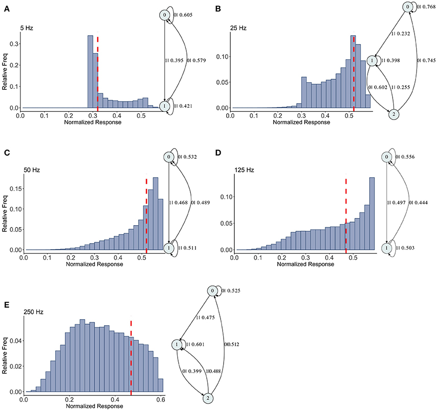
Figure 6. Causal state machines (CSMs) reconstructed and their corresponding relative frequency distributions obtained from mixed FD model driven by a Poisson spike train with mean rates (A) 5, (B) 25, (C) 50, (D) 125, and (E) 250 Hz. In (A,C,D), CSMs for mean firing rates of 5, 50, and 125 Hz consist of two states with similar structure, emitting successive large responses followed by small responses. 3-State CSM for mean firing rate 25 Hz has more complex graph structure. Note that this is inflection point for this synapse model (see Figure 1).

The hierarchy of the machines for each set of parameter values is evident, and it is possible to visualize transformations of one machine into another as the firing rate is changed. To sum up these results we plot the statistical complexity of the machines as a function of frequency in each case. See Figure 7. We now seek to connect this back to properties of the synapse model itself.

FIGURE 7

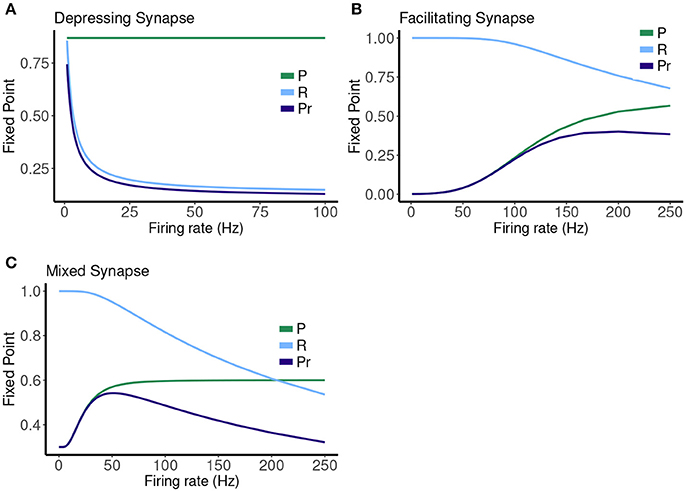
Figure 7. Fixed point values for release probability P, fraction of readily releasable pool R and normalized postsynaptic response Pr for varying mean firing rates ranges from 0.1 to 100 Hz for (A) depressing synapse and from 0.1 to 250 Hz for (B) facilitating and (C) mixed synapse.

4. Discussion: Interpretation of Results

The depressing synapse is the simplest of the three cases, and through this investigation it is clear that the formulation of the distribution of the Pr in terms of the “stochastic fixed point” gives an almost entire description of the dynamics. For very small and very large frequencies the data points are almost all 1's or 0's, respectively, so the machine has one state. In the small frequency range where the distribution slides from being concentrated at P_max to be concentrated at zero, the epsilon machine shows that the dynamics are still simple, and can be explained by two causal states, one with mostly 0's and the other with mostly 1's. Changing frequency affects the transition probabilities on the edges only.

The other two cases are much less simple. More complicated dynamics are possible as the input firing changes. The complexity of the machines for the facilitating synapse compared to the depressing and mixed synapse can be understood by comparing the “decomposed” fixed point spectrum. See Figure 8. Plotting the fixed points in R and P along with Pr shows a striking difference between the three cases. The depressing synapse Pr fixed point is entirely controlled by the variation in R, as P remains constant over the range of frequencies, and the P variation happens in a very small range of frequencies near zero. The facilitating synapse has a range of R-values across the spectrum, as well as a range of P-values. The mixed synapse has a very little variation in P. The more complicated machines in both cases occur at frequencies where there is the largest variation in both. Obviously, having a range of response in both P and R creates the complexity of the machines, however indirectly.

FIGURE 8

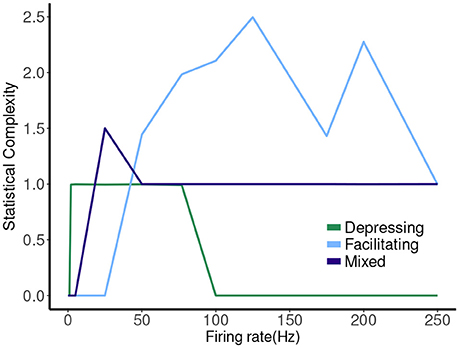
Figure 8. Statistical complexity values obtained from average amount of information of the distribution over causal states as a function of mean firing rates for synapse models, “depressing,” “facilitating,” and “mixed”.

Another way to view this difference is through the calcium decay time. For the depressing synapse τ_ca is very short, and there is very little correlation in the calcium time series in all but very high frequencies (which are not physiological). The synapse simply filters the Poisson spike train process. In the mixed case, while the calcium time series is more correlated, the lack of variation of the P response flattens out any downstream effect on Pr. The facilitating case is really in the “goldilocks zone” where the correlation in the calcium time series can effect Pr through the variation in P. A synapse might be expected to be a more complex filter if there is a hidden time dependent variable, such as calcium, that links the two processes of facilitation and depression, as it does in this model for larger τ_ca or higher frequencies. The exact details of the relationship between the probability of release, and the rate of recovery of R as they depend upon C must line up to produce sensitivity in the fixed point values for each in the same frequency range.

Finally, we note that the histograms themselves, from which many information measures are constructed, do not tell the whole story. There is a much more complicated dynamic occurring in the facilitating synapse than the depressing synapse, though comparing the histograms themselves in the two cases does not suggest this. We have also seen the converse, where the machines are the same, even though the distributions are quite different. This implies that both are needed to have a full understanding of such a stochastic process.

5. Conclusions

In this paper we demonstrate the validity of using causal state models to more completely describe stochastic short-term synaptic plasticity. These models rely only upon output data from a synaptic connection, knowledge of the input stimulus stream is not required. This will expand the arena of experiments where data can directly inform models, and more importantly uses the data itself to create models. While these models are not physiologically motivated per se, we have shown how we can connect the structure of the model to complexity of the mechanisms involved, a useful first step in a more complete categorization of short term plasticity. Interpreting synaptic plasticity in the language of computation could also be exploited in the construction of large scale models of neural processes involving many thousands of neural connections, and potentially lead to a more complete theoretical description of the computations possible.

Our results also draw direct connections between the causal state models and the deterministic dynamics of the underlying model used to create the data. Specifically, they point to the importance of having variability in both probability of release and the recovery rate of resources with frequency in creating a more complex synaptic filter. This finding can be reversed (at some peril, we realize) to imply that a more complicated machine results from a synapse with such variability. This in turn could be used to inform the development of physiologically accurate models, or direct future experimental design. Interested reader may receive any/all of the code use to create these results by contacting Elham Bayat-Mohktari.